Lattices

We work on regular hypercubic lattices in \(D\) dimensions with \(N\) sites per direction and periodic boundary conditions.

Note

The lattice is specified by a single \(N\): every direction has the same number of sites. This equal-size (hypercubic) assumption is baked into much of the code — modular arithmetic on coordinates, the Fourier-transform and correlation helpers, and observables that normalize by a length or volume (for example VortexSusceptibilityScaled, which scales by \(N^{D}\)). Anisotropic lattices with a different number of sites in different directions are not supported.

The Interlaced Picture

Fields do not only live on sites. A scalar field assigns a value to every site, but a gauge field assigns a value to every link, a field strength to every plaquette, and so on: a \(p\)-form (see Differential Forms) assigns a value to every \(p\)-dimensional cell of the lattice.

Every cell has a natural geometric location. A site sits at integer coordinates \(n = (n_0, \ldots, n_{D-1})\). The link leaving \(n\) in direction \(k\) is centered half a step away, at \(n + \hat{e}_k/2\). The plaquette anchored at \(n\) spanning directions \(j\) and \(k\) is centered at \(n + (\hat{e}_j + \hat{e}_k)/2\). In general, the \(p\)-cell anchored at \(n\) spanning the directions \(I = (i_1 < i_2 < \cdots < i_p)\) is centered at \(n + \frac{1}{2} \sum_{i \in I} \hat{e}_i\).

Doubling every coordinate clears the half-integers. Measured in half-lattice units, the cell anchored at \(n\) spanning the directions \(I\) sits at

\[x = 2n + \mathbb{1}_I\]

where \(\mathbb{1}_I\) has a 1 in the directions the cell spans and a 0 elsewhere. Now every cell of every degree occupies a distinct integer point of a \((2N)^D\) lattice, and the parity of the coordinates says what kind of cell lives there: \(x_k\) is odd exactly when the cell extends in direction \(k\). A \(p\)-cell is a point with exactly \(p\) odd coordinates, and its anchoring site is always \(n = \lfloor x/2 \rfloor\).

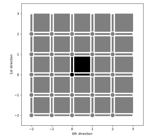
We call this doubled lattice interlaced because the cells of every degree are interleaved on a single grid. The figure below shows the four cells anchored at the origin of a two-dimensional lattice: the site at interlaced coordinates \((0,0)\), the two links at \((1,0)\) and \((0,1)\), and the plaquette at \((1,1)\).

(Source code, png, hires.png, pdf)

The interlaced picture is how the code “thinks” geometrically: which cells are incident to which, which neighbor a value is gathered from, and where the operators of the exterior calculus get their shifts and signs. The storage, however, is compact: a point with exactly \(p\) odd coordinates is rare (only \(\binom{D}{p}/2^D\) of the doubled lattice), so a \(p\)-form is stored as an array of shape \((\binom{D}{p}, N, \ldots, N)\) whose 0th axis enumerates the components — the sorted direction tuples \(I\), in lexicographic order — and whose remaining axes give the anchoring site \(n\). See Form.

A reference implementation that stores forms directly as sparse \((2N)^D\) interlaced arrays is documented with the other reference implementations. But even on small 4-dimensional lattices the interlaced representation is much slower than the compact representation, so we use the compact representation for all practical purposes.

Arbitrary Dimensions

We provide common machinery for working with (hyper)cubic lattices in arbitrary dimensions. For some purposes (like plotting) it is useful to have a specialization; for example below we provide Lattice2D for two dimensions.

class supervillain.lattice.Lattice(D, N)

A D-dimensional hypercubic lattice with N sites per direction.

The lattice knows how to enumerate the components of any p-form and can create zero or random p-forms on demand.

to_h5(group, _top=True)

Write D and N to HDF5; everything else is recomputed on load.

classmethod from_h5(group, strict=True, _top=True)

Reconstruct from HDF5 by reading D and N reconstructing the rest.

property sites

Total number of sites \(N^D\).

property dims

Tuple of side lengths (N, N, …, N), length D.

property origin

The origin site \((0, \ldots, 0)\), a tuple of length \(D\). Use it to index the zero-displacement element of a scalar field or correlator of shape \((N,)^D\) (e.g. correlator[lattice.origin]) without assuming \(D=2\). A Form has a leading component axis, so index the component first: form[c][lattice.origin].

property dim

Number of dimensions (alias for D).

property links

Total number of links (1-form components) \(D N^D\).

property cells_of_degree

p → number of p-cells = \(C(D,p) N^D\).

Type

dict[int, int]

property cells_of_codegree

q → number of (D−q)-cells = \(C(D, D−q) N^D\).

Type

dict[int, int]

property coords

FFT-convention coordinate for each lattice site, shape (D, N, …, N).

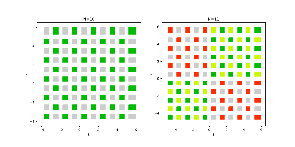
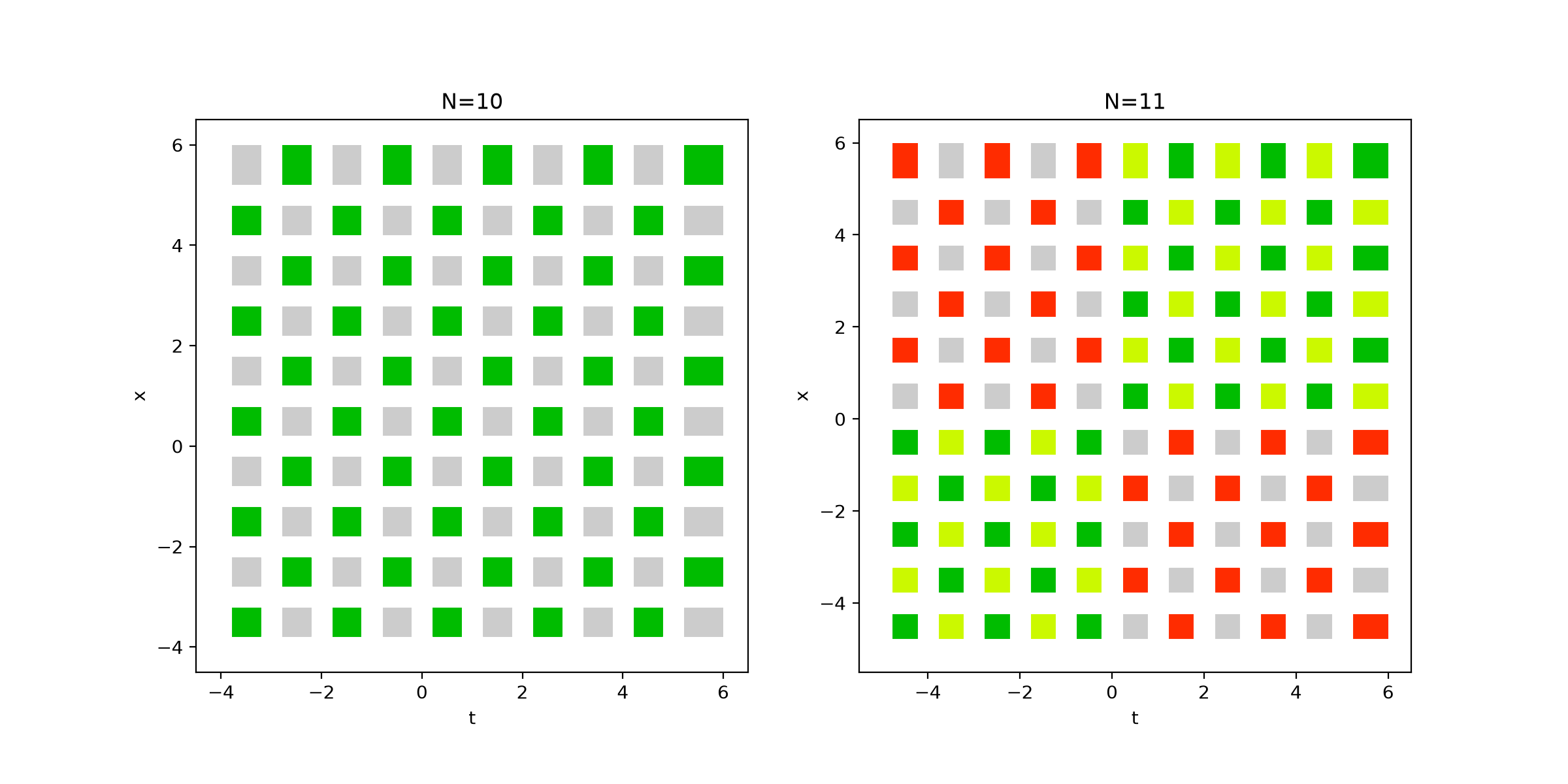
property checkerboarding

Partition lattice sites into colors with no same-color nearest neighbors.

On a lattice of even size both the sites and plaquettes can be bipartitioned so that no simplex of one color has a neighbor of the same color. On an odd-sized lattice the periodic boundary conditions make it impossible to accomplish this with only 2 colors, but a similar construction with more colors is possible.

With even \(N\) there are two colors (coordinate-sum parity); with odd \(N\) there are \(2^{\max(D, 2)}\) to ensure that no nearest-neighbor sites share a color. The figure below shows both cases for D=2:

(Source code, png, hires.png, pdf)

Returns

• tuple of index-array tuples – One np.where result per color; each element selects that color’s sites from the D spatial axes of a form:

  for i, color in enumerate(L.checkerboarding):
      form[(slice(None), *color)] = i
  

• .. warning:: – No promise is made about the future sizes of the color partitions. For example, it might be wiser for performance to split the odd-N colors less evenly. All that is promised is that within each color no site shares a nearest-neighbor edge with a site of the same color.

zeros(p, dtype=<class 'float'>)

Return a zero p-form.

Parameters

• p (int) – Form degree.

• dtype (data-type, optional) – np dtype for the underlying array (default float).

Returns

Zero p-form of shape (C(D,p), N,...,N).

Return type

Form

random(p)

Return a p-form with entries drawn uniformly from [0, 1).

Parameters

p (int) – Form degree.

Returns

Random p-form of shape (C(D,p), N,...,N).

Return type

Form

form(p, dtype=<class 'float'>)

Return a zero p-form.

Alias for zeros().

Parameters

• p (int) – Form degree.

• dtype (data-type, optional) – NumPy dtype (default float).

Returns

Zero p-form of shape (C(D,p), N,...,N).

Return type

Form

property R_squared

Distance-squared from the origin at each site, shape (N,…,N).

distance_squared(a, b)

Squared lattice distance between coordinate vectors a and b.

Accounts for periodic boundary conditions: the distance is computed via mod(a - b), so it is the shortest-path distance on the torus.

Parameters

a, b (array_like) – Coordinate vectors of shape (D,) for a single pair, or (..., D) for a batch.

Returns

Scalar for a single pair, shape (...) for a batch.

Return type

np.ndarray

property coordinates

Array of shape (sites, D) listing every site’s coordinates.

mod(x)

Map integer coordinates into FFT-convention lattice values.

Parameters

x (array_like) – Integer site coordinates (any shape).

Returns

Coordinates in the range [-(N//2), N//2) (FFT convention).

Return type

np.ndarray

fft(form, axes=None)

D-dimensional DFT over the spatial axes of form.

\[F_{\boldsymbol{k}} = \frac{1}{N^{D/2}} \sum_{\boldsymbol{x}} e^{-2\pi i \boldsymbol{k}\cdot\boldsymbol{x}/N} f_{\boldsymbol{x}}\]

Parameters

• form (np.ndarray) – The data to transform. Spatial axes are the last D axes.

• axes (tuple of int, optional) – Override which axes to transform. Defaults to the last D axes.

Returns

The Fourier-transformed array (complex).

Return type

np.ndarray

ifft(form, axes=None)

D-dimensional inverse DFT over the spatial axes of form.

Parameters

• form (np.ndarray) – The data to transform. Spatial axes are the last D axes.

• axes (tuple of int, optional) – Override which axes to transform. Defaults to the last D axes.

Returns

The inverse-Fourier-transformed array (complex).

Return type

np.ndarray

convolution(f, g, axes=None)

The convolution is given by

\[\texttt{convolution}(f,g)(\boldsymbol{r}) = (f * g)(\boldsymbol{r}) = \sum_{\boldsymbol{x}} f(\boldsymbol{x})\,g(\boldsymbol{r}-\boldsymbol{x})\]

The convolution is Fourier accelerated.

With the ortho-normalized DFT convention \(f(\boldsymbol{x}) = N^{-D/2} \sum_{\boldsymbol{k}} F_{\boldsymbol{k}}\, e^{2\pi i\,\boldsymbol{k}\cdot\boldsymbol{x}/N}\),

\[\begin{split}\begin{aligned} (f * g)(\boldsymbol{r}) &= \sum_{\boldsymbol{x}} \Bigl(\tfrac{1}{N^{D/2}}\sum_{\boldsymbol{k}} F_{\boldsymbol{k}}\, e^{2\pi i\,\boldsymbol{k}\cdot\boldsymbol{x}/N}\Bigr) \Bigl(\tfrac{1}{N^{D/2}}\sum_{\boldsymbol{k}'} G_{\boldsymbol{k}'}\, e^{2\pi i\,\boldsymbol{k}'\cdot(\boldsymbol{r}-\boldsymbol{x})/N}\Bigr) \\ &= \frac{1}{N^D}\sum_{\boldsymbol{k},\boldsymbol{k}'} F_{\boldsymbol{k}} G_{\boldsymbol{k}'}\, e^{2\pi i\,\boldsymbol{k}'\cdot\boldsymbol{r}/N} \underbrace{ \sum_{\boldsymbol{x}} e^{2\pi i\,(\boldsymbol{k}-\boldsymbol{k}')\cdot\boldsymbol{x}/N} }_{N^D\,\delta_{\boldsymbol{k}\boldsymbol{k}'}} \\ &= \sum_{\boldsymbol{k}} F_{\boldsymbol{k}} G_{\boldsymbol{k}}\, e^{2\pi i\,\boldsymbol{k}\cdot\boldsymbol{r}/N} \\ &= \sqrt{N^D}\times \underbrace{\tfrac{1}{N^{D/2}}\sum_{\boldsymbol{k}} \bigl(F_{\boldsymbol{k}} G_{\boldsymbol{k}}\bigr)\, e^{2\pi i\,\boldsymbol{k}\cdot\boldsymbol{r}/N} }_{\texttt{ifft}(\hat f \hat g)(\boldsymbol{r})} \\ \texttt{convolution}(f,g) &= \sqrt{N^D}\;\texttt{ifft}\!\bigl(\texttt{fft}(f)\cdot\texttt{fft}(g)\bigr) \end{aligned}\end{split}\]

Parameters

• f, g (np.ndarray) – Forms on this lattice; spatial axes are the last D axes.

• axes (tuple of int, optional)

Return type

np.ndarray

correlation(f, g, axes=None)

The cross-correlation is given by

\[\texttt{correlation}(f,g)(\boldsymbol{r}) = (f \star g)(\boldsymbol{r}) = \frac{1}{N^D} \sum_{\boldsymbol{x}} f(\boldsymbol{x})^*\,g(\boldsymbol{x}-\boldsymbol{r})\]

where \(f^*\) is the complex conjugate of \(f\).

The cross-correlation is Fourier accelerated.

With the ortho-normalized DFT convention \(f(\boldsymbol{x}) = N^{-D/2} \sum_{\boldsymbol{k}} F_{\boldsymbol{k}}\, e^{2\pi i\,\boldsymbol{k}\cdot\boldsymbol{x}/N}\),

\[\begin{split}\begin{aligned} (f \star g)(\boldsymbol{r}) &= \frac{1}{N^D}\sum_{\boldsymbol{x}} \Bigl(\tfrac{1}{N^{D/2}}\sum_{\boldsymbol{k}} F_{\boldsymbol{k}}\, e^{2\pi i\,\boldsymbol{k}\cdot\boldsymbol{x}/N}\Bigr)^* \Bigl(\tfrac{1}{N^{D/2}}\sum_{\boldsymbol{k}'} G_{\boldsymbol{k}'}\, e^{2\pi i\,\boldsymbol{k}'\cdot(\boldsymbol{x}-\boldsymbol{r})/N}\Bigr) \\ &= \frac{1}{N^{2D}}\sum_{\boldsymbol{k},\boldsymbol{k}'} F_{\boldsymbol{k}}^* G_{\boldsymbol{k}'}\, e^{-2\pi i\,\boldsymbol{k}'\cdot\boldsymbol{r}/N} \underbrace{ \sum_{\boldsymbol{x}} e^{2\pi i\,(\boldsymbol{k}'-\boldsymbol{k})\cdot\boldsymbol{x}/N} }_{N^D\,\delta_{\boldsymbol{k}\boldsymbol{k}'}} \\ &= \frac{1}{N^D}\sum_{\boldsymbol{k}} F_{\boldsymbol{k}}^* G_{\boldsymbol{k}}\, e^{-2\pi i\,\boldsymbol{k}\cdot\boldsymbol{r}/N} \\ &= \frac{1}{\sqrt{N^D}}\times \underbrace{\tfrac{1}{N^{D/2}}\sum_{\boldsymbol{k}} \bigl(F_{\boldsymbol{k}}^* G_{\boldsymbol{k}}\bigr)\, e^{-2\pi i\,\boldsymbol{k}\cdot\boldsymbol{r}/N} }_{\texttt{fft}(\hat f^*\!\cdot\hat g)(\boldsymbol{r})} \\ \texttt{correlation}(f,g) &= \texttt{fft}\!\bigl(\texttt{fft}(f)^*\cdot\texttt{fft}(g)\bigr) / \sqrt{N^D} \end{aligned}\end{split}\]

Warning

We have \(g(\boldsymbol{x}-\boldsymbol{r})\) whereas Wikipedia has \(g(\boldsymbol{x}+\boldsymbol{r})\). The difference is just the sign of the relative coordinate.

Warning

We normalize by the spacetime volume \(N^D\); Wikipedia does not.

Parameters

• f, g (np.ndarray) – Forms on this lattice; spatial axes are the last D axes.

• axes (tuple of int, optional)

Return type

np.ndarray

linearize(v, dims=(-1,))

Flatten the D spatial dims of v into a single axis of size sites.

Parameters

• v (np.ndarray) – Array whose D adjacent spatial dims will be collapsed into one.

• dims (tuple of int) – Axes of the result that come from flattening. Pass the same value to coordinatize() for a round-trip.

Return type

np.ndarray

coordinatize(v, dims=(-1,), center_origin=False)

Unflatten a linear site-index axis back into D spatial axes.

Parameters

• v (np.ndarray) – Array with a sites-sized axis to expand.

• dims (tuple of int) – Axes of v to unflatten. Each must have size sites.

• center_origin (bool) – If True, roll each spatial block so that the origin sits in the centre of the array. Useful for visualisation; not invertible.

Return type

np.ndarray

symmetrize(correlator, dims=(-1,))

Average correlator over the hyperoctahedral group (D!·2^D signed permutations).

Projects onto the totally-symmetric (A₁/trivial) irrep of the lattice point group.

(Source code, png, hires.png, pdf)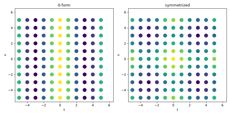

Parameters

• correlator (np.ndarray) – Spatial shape (N,...,N) (or any array whose dims axes span the sites of this lattice after linearization).

• dims (tuple of int) – Axes to symmetrize (same convention as linearize()).

Returns

Same shape as correlator.

Return type

np.ndarray

Two Dimensions

class supervillain.lattice.Lattice2D(n)

A two-dimensional square lattice — a thin wrapper around Lattice with D=2.

All lattice machinery (forms, exterior derivative, codifferential, Fourier transforms, symmetrize, linearize/coordinatize, …) is inherited from Lattice. Lattice2D adds only the plot_form() visualisation helper and the nt/nx aliases.

Parameters

n (int) – The number of sites on a side.

classmethod from_h5(group, strict=True, _top=True)

Reconstruct from HDF5 by reading D and N reconstructing the rest.

property plaquettes

\(C(2,2) N^2 = N^2\).

Type

Number of plaquettes (2-cells)

property nt

Temporal extent N.

property nx

Spatial extent N.

property t

FFT-convention t-coordinates (first direction), shape (N,).

property x

FFT-convention x-coordinates (second direction), shape (N,).

property T

Array of shape (N, N) with the t-coordinate at each site.

property X

Array of shape (N, N) with the x-coordinate at each site.

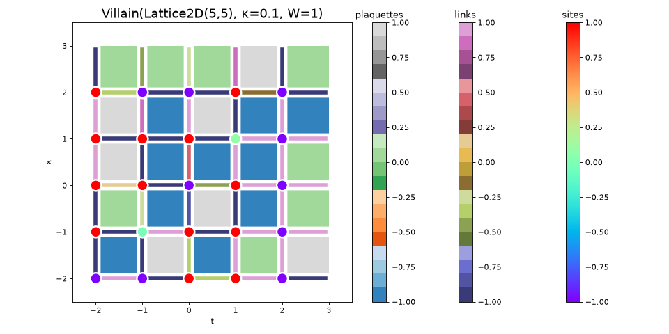
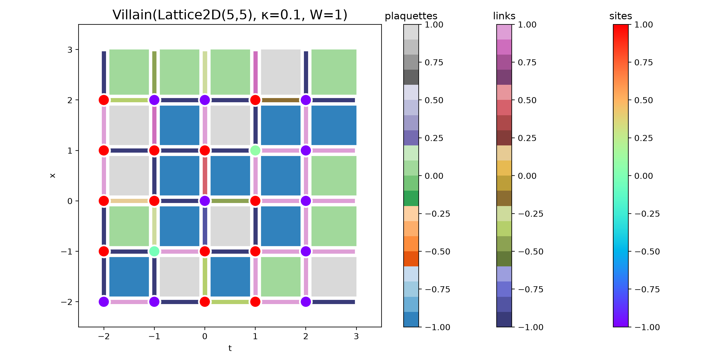
plot_form(form, axis, label=None, zorder=None, cmap=None, cbar_kw={}, norm=<matplotlib.colors.CenteredNorm object>, pointsize=200, linkwidth=0.025, background='white', markerstyle='o')

Plots the form on the axis. The degree of the form determines whether sites, links, or plaquettes are visualized.

The following figure shows a 0-form plotted on sites, a 1-form on links, and a 2-form on plaquettes. See the source for details.

(Source code, png, hires.png, pdf)

Parameters

• form (Form) – The p-form to plot; form.degree determines the visualization.

• axis (matplotlib.pyplot.axis) – The axis on which to plot.

Returns

A handle for the data-sensitive part of the plot.

Return type

matplotlib.image.AxesImage

Other Parameters

• label (string) – If specified, show a colorbar with the title given by the label.

• zorder (float) – If None defaults to -form.degree to layer plaquettes, links, and sites well.

• cmap (string or matplotlib.colors.Colormap) – If a string, it should name a colormap known to matplotlib.

• cbar_kw (dict) – A dictionary of keyword arguments forwarded to the colorbar constructor.

• norm (matplotlib.colors.Normalize) – A matplotlib color normalization.